
What do you know about the Population Stability Index (PSI) measure, its historical usage, and its connection to other mathematical drift measures such as KL divergence? PSI is a widely used tool for detecting data drift, helping organizations monitor shifts in data distributions over time. If you’re left scratching your head, don’t worry — we’ve got you covered!
What is the Population Stability Index (PSI)?
PSI is a commonly used measure in the financial services domain to quantify the shift in the distribution of a variable over time. While several resources give an overview of PSI, such as this visual blog by Matthew Burke and this paper summary [3], they often do not discuss the connection between PSI as a drift metric and other popular measures such as KL divergence.

Briefly, the PSI metric is calculated based on the multinomial classification of a variable into bins or categories. Consider two distributions shown in the left figure above. These distributions can be converted into their respective histograms with an appropriately chosen binning strategy. There are several binning strategies, and each strategy can yield varying PSI values. For the figure on the right, data is collected in equi-width bins, producing a histogram that resembles a discretized version of the respective PSI distribution. Another possible binning strategy is equi-quantiles or equi-depth binning. In this case, each bin would have the same proportion of samples in the reference / expected distribution. The choice of the strategy is context-specific and requires domain knowledge. For example, in credit score monitoring, credit scores are already binned into ranges representing a client's credit risk. In such cases, it may be desirable to use consistent binning throughout the analysis
The differences in each bin between the expected distribution (AKA reference or initial distribution) and the target distribution (AKA new or actual distribution) are then utilized to calculate PSI as follows:
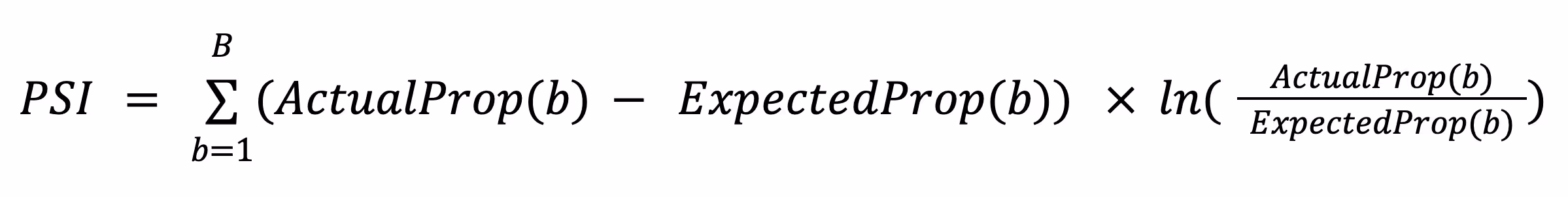
Where, \(B\) is the total number of bins, \(ActualProp(b)\) is the proportion of counts within bin \(b\) from the target distribution and \(ExpectedProp(b)\) is the proportion of counts within bin \(b\) from the reference distribution. Thus, PSI is a number that ranges from zero to infinity and has a value of zero when the two distributions exactly match.
Practical Notes: The rules of thumb in practice regarding PSI thresholds are that if: (1) PSI is less than 0.1, then the actual and the expected distributions are considered similar, (2) PSI is between 0.1 and 0.2, then the actual distribution is considered moderately different from the expected distribution, and (3) PSI is beyond 0.2, then it is highly advised to develop a new model on a more recent sample [1,2]. Also, since there is a possibility that a particular bin may be empty, PSI can be numerically undefined or unbounded. To avoid this, in practice, a small value such as 0.01 can be added to each bin proportion value. Alternatively, a base count of 1 can be added to each bin to ensure non-zero proportion values.
PSI Usage History and Applications
PSI is typically used in financial services as a guidepost to compare current to baseline populations for which some financial tool or service was developed. For example, the use of credit scoring tools has proliferated in the banking industry to evaluate the level of credit risk associated with applicants or customers. Such tools provide statistical odds or probabilities that an applicant with a given credit score will pay off their credit. In the context of credit scoring, it is crucial to study the effects of changing populations or irregular trends in application approval rates. Similarly, abnormal periods where the population may under- or over-apply in line with regular business cycles are also important. PSI helps quantify such changes and provides a basis to the decision-makers that the development sample is representative of future expected applicants. Identifying distributional change can significantly impact the maintenance of tools capable of accurate lending decisions.
While there are no explicit resources that we found on the rationale of using PSI, we conjecture that PSI usage stems from multiple factors as listed below:
- Regulations such as Basel Accords and the International Financial Reporting Standards (IFRS 9) discuss assessing the risk of loans with three components: the probability of default (PD), exposure at default (EAD), and loss given default (LGD). Since PSI measures shifts in probability distributions, its usage for measuring shifts in PD seems likely due to such regulations.
- PSI uses binning of variables, including numerical variables, which implies categorizing variables into bins. Despite being a numerical quantity, credit scores are typically categorized into bins in the financial sector. Such a practice also points towards the ease of usage of PSI within the industry.
- The PSI metric may have been widely adopted due to its inclusion in popular software such as SAS® Enterprise Miner™.
With the ongoing adoption of machine learning models and systems in financial services, PSI has gained popularity as a model monitoring metric — we only expect this trend to continue as model portfolios grow and the MLOps lifecycle becomes standardized within organizations.
Understanding the PSI Formula and Its Connection to KL Divergence
The Kullback-Leibler divergence or relative entropy is a statistical distance measure that describes how one probability distribution is different from another.
Given two discrete probability distributions \(A\) (actual), and \(E\) (expected) defined on the same probability space, KL divergence is defined as:
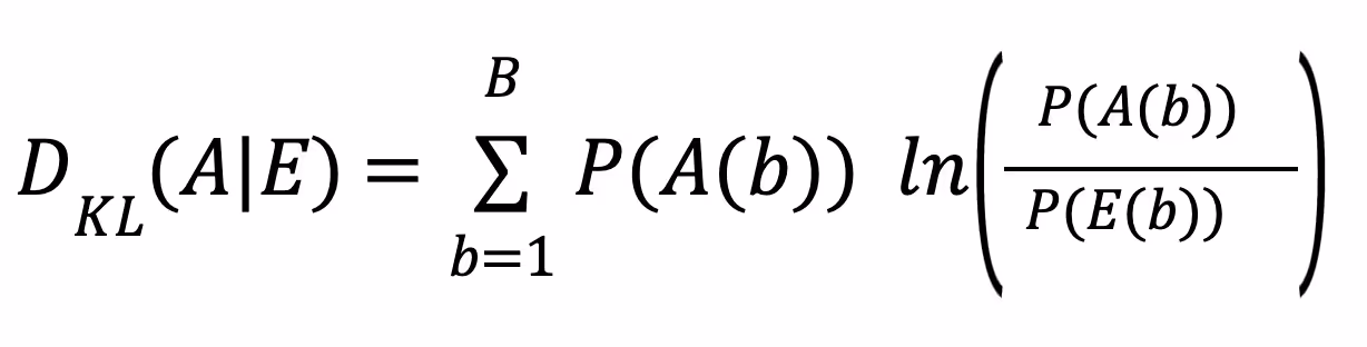
An interpretation of KL divergence is that it measures the expected excess surprise in using the actual distribution versus the expected distribution as a divergence of the actual from the expected. This sounds a lot like the reasoning behind using PSI! While KL divergence is well studied in mathematical statistics [4] and has a lot of references to academic work [1,2], PSI is domain-specific and lacks concrete literature on the history of its usage within financial services. In the following, we illustrate how PSI can actually be viewed as a special form of KL divergence.
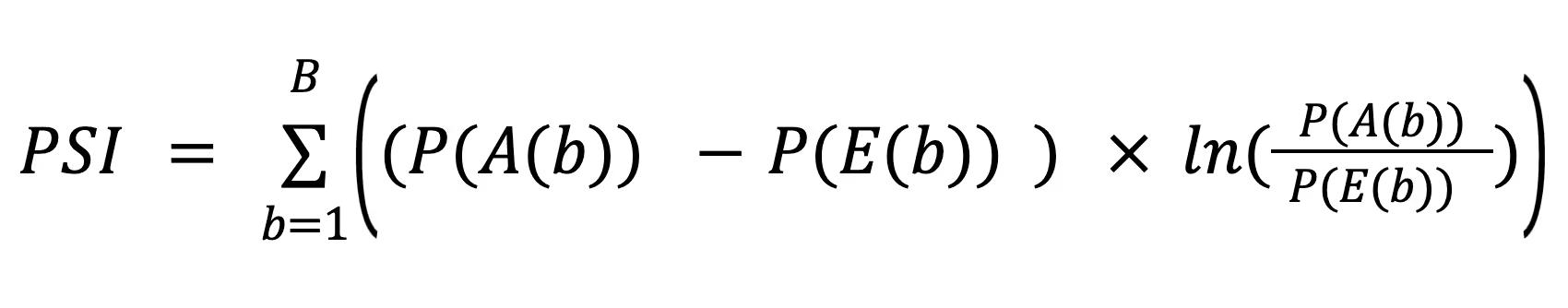
Consider the PSI formula and let us look at the proportion of counts within a bin b for the actual distribution \(ActualProp(b)\) as the frequentist probability \(PA(b)\) of the variable appearing in that bin. The same applies to the expected distribution.
Then, we can rewrite the PSI formula as:
On expanding further,
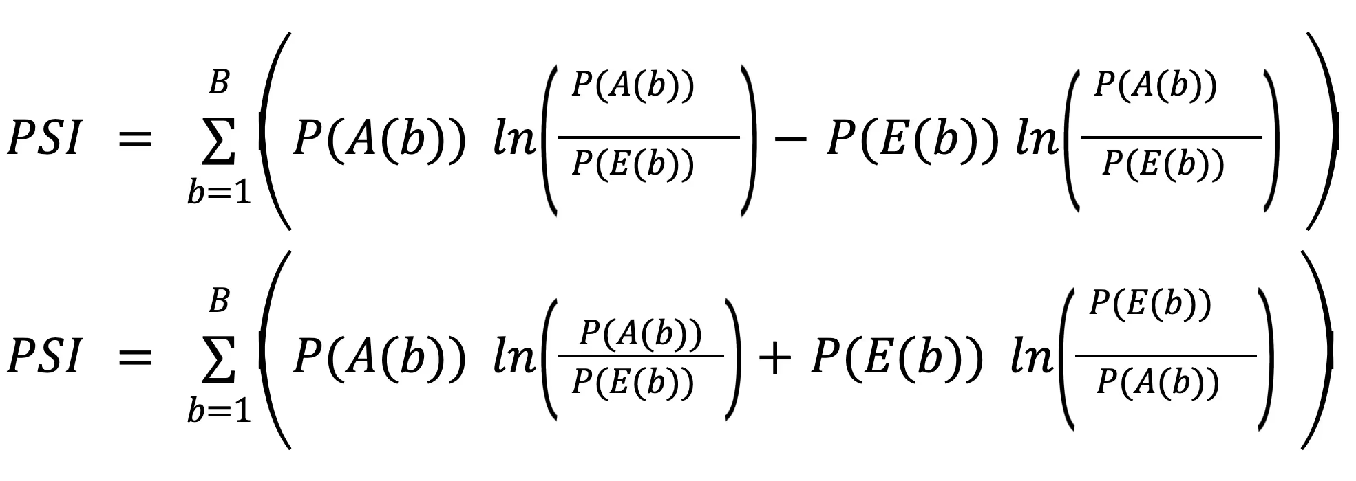
Thus, PSI can be rewritten as:
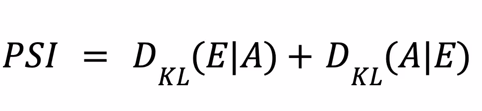
which is the symmetrized KL divergence!
We hope you enjoyed this overview of PSI. Don’t forget to check out our blog on detecting intersectional unfairness in AI!
Enhance Data Drift Detection with Fiddler’s Analytics
Fiddler’s analytics features provide the tools needed to detect and analyze data drift precisely. Build custom reports to gain deeper insights into your models, from monitoring PSI metrics, feature impact, and correlation to tracking PSI distribution changes and visualizing Partial Dependence Plot (PDP) charts. With Fiddler, you can proactively monitor model performance and ensure reliable business outcomes.
———
References
- Siddiqi, N. (2017). Intelligent credit scoring: Building and implementing better credit risk scorecards. John Wiley & Sons.
- Yurdakul, B. (2018). Statistical properties of population stability index. Western Michigan University.
- Lin, A. Z. (2017). Examining Distributional Shifts by Using Population Stability Index (PSI) for Model Validation and Diagnosis. SAS Conference Proceedings: Western Users of SAS Software 2017 September 20-22, 2017, Long Beach, California URL https://www.lexjansen.com/wuss/2017/47_Final_Paper_PDF.pdf
- Kullback, S., & Leibler, R. A. (1951). On Information and Sufficiency. The Annals of Mathematical Statistics, 22(1), 79–86. http://www.jstor.org/stable/2236703