
ML teams often understand the importance of monitoring model performance as part of the MLOps lifecycle, but may not know what to monitor or the “hows”:
- How model performance is measured for the most common types of ML models
- How to catch data pipeline errors before they affect your models, as part of feature quality monitoring
- How to detect when real-world data distribution has shifted, causing your models to degrade in performance
- How to monitor unstructured Natural Language Processing and Computer Vision models and the unique challenges this entails
- How to address the common problem of class imbalance and what it means for model monitoring
But before we dive into those, we need to consider why ML models are different from traditional software and how this affects your monitoring framework.
ML models are not like traditional software
Traditional software uses hard-coded logic to return results; if software performs poorly, you know there’s likely a bug somewhere in the logic. In contrast, ML models leverage sophisticated statistical analyses of inputs to predict outputs. And when models start to misbehave, it can be far less clear as to why. Has the ingested production data shifted from the training data? Is the upstream data pipeline itself broken? Was your training data too narrow for the production use case? Is there potential model bias at play?
Why monitoring model performance is important
ML models tend to fail silently and over time. They don’t throw errors or crash like traditional software. Without continuous model monitoring, teams are in the dark when a model starts to make inaccurate predictions, potentially causing major impact. Uncaught issues can damage your business, harm your end-users, or even violate AI regulations or model compliance rules.
How to measure model performance
Model performance is measured differently based on the type of model you’re using. Some of the most common model types are:
- Classification models - Categorize inputs into one or more buckets, for example a model that classifies loans as low, medium, or high risk. Classification models can be binary or multi-class.
- Regression models - Use complex analyses to model the relationships between inputs and output, for example models that forecast trends.
- Ranking models - Return a ranking based on inputs, for example recommendation systems used for search results.
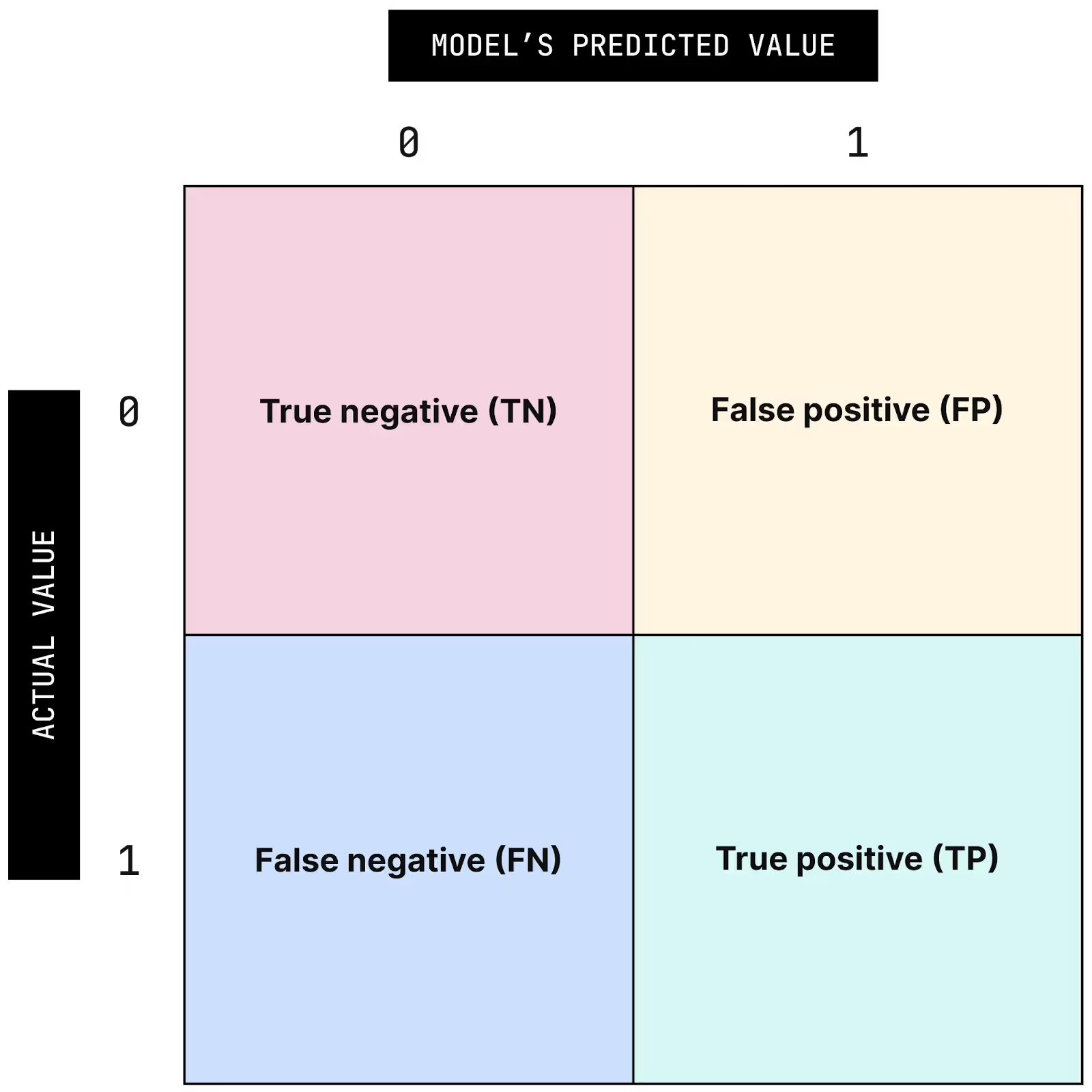
Classification models
Before we go into performance metrics for classification models, it’s worth referencing the basic terminology behind “true” or “false” positives and negatives, as represented in a confusion matrix:
Even though the following metrics are being presented for binary classification models, they can also be extended to multi-class models, with appropriate weighting if dealing with imbalanced classes (more on this later).
Accuracy
Accuracy captures the fraction of predictions your model got right:
$$ACC = \frac{TP+TN}{TP + FP+TN+FN}$$
But if your model deals with imbalanced data sets, accuracy can be deceiving. For instance, if the majority of your inputs are positive, you could just classify all as positive and score well on your accuracy metric.
True positive rate (recall)
The true positive rate, also known as recall or sensitivity, is the fraction of actual positives that your model classified correctly.
$$TPR = \frac{TP}{TP + FN}$$
If you can’t miss inputs that your model should have classified correctly, recall is a great metric to optimize. For a use case like fraud detection, recall would likely be one of your most important metrics.
False positive rate
Want to know how often your model classifies something as positive when it was actually negative? You need to calculate your false positive rate.
$$FPR = \frac{FP}{FP + TN}$$
Sticking with the fraud detection example, though you may care more about recall than false positives, at a certain point you risk losing customer or team confidence if your model triggers too many false alarms.
Precision
Also called “positive predictive value,” precision measures how many inputs your model correctly classified as positive.
$$PPV = \frac{TP}{TP + FP}$$
Precision is often used in conjunction with recall. Increasing recall likely decreases precision, because your model becomes less choosy. This, in turn, increases your false positive rate!
F1 score
F1 score is used as an overall metric for model quality. It is the harmonic mean of precision and recall; mathematically, it combines both into one metric.
$$F_{1} = \frac{2}{recall^{-1} + precision^{-1}} = 2 \frac{precision * recall}{precision + recall} = \frac{TP}{TP + \frac{1}{2}{(FP+FN)}}$$
A high F1 score indicates your model not only has good coverage, but also makes few errors.
Area under curve (AUC)
Considered a key metric for classification models, AUC visualizes how your model is performing. It plots the true positive rate (TPR) against the false positive rate (FPR).

Ideally, your model has a high area under the curve, indicating it has a very high recall compared to a very low false positive rate.
Now that we’ve scratched the surface of model performance metrics for classification models, read our entire Ultimate Guide to Model Performance to become an expert on everything model performance, including:
- Performance metrics for regression and ranking models
- Feature quality monitoring to catch data pipeline errors early
- What model drift is and how to measure it
- How to measure the performance of models that ingest unstructured data, like natural language processing and computer vision models
- The ways class imbalance can affect performance monitoring and how to solve for it