
In this blog, we discuss how explanations of Computer Vision (CV) model predictions can be made more human-centric and also address a criticism of the approach used to generate such model explanations, namely Integrated Gradients (IG). We show that for two randomly initialized weights and biases (model parameters) for a specific model architecture, a heatmap (saliency map) that explains which regions of the image the model is paying attention to, appear to be visually similar. However, the same does not hold true for the model loaded with trained parameters. Randomization of model parameters is discussed as an approach in existing literature as a way to evaluate the usefulness of explanation approaches such as IG. From the perspective of such a test, since the explanations for two randomly initialized models appear similar, the approach doesn’t seem useful. However, we highlight that IG explanations are faithful to the model, and dismissing an approach due to the results of two randomly initialized models may not be a fair test of the explanation method. Furthermore, we discuss the effects of the post-processing decisions such as normalization while producing such maps and its impact on visual bias between two images overlaid with their respective IG attributions. We see that the pixel importance (min-max attribution values) of both images that are being compared, need to be utilized for the post-processing of heatmaps to fairly represent the magnitudes of the impact of each pixel across the images. If the normalization effects aren't clarified to the user, human biases during the visual inspection of two heatmaps may result in a misunderstanding of the attributions.
Computer Vision and Explainable AI
Computer Vision (CV) is a fascinating field that delves into the realm of teaching computers to understand and interpret visual information. From recognizing objects in images to enabling self-driving cars, CV has revolutionized how machines perceive the world. And at the forefront of this revolution lies Deep Learning, a powerful approach that has propelled CV to new heights. However, as we explore the possibilities of this technology, we must also address the need for responsible and explainable AI.
Explainable AI (XAI) aims to shed light on the inner workings of AI models1-5. Particularly in the field of Computer Vision, XAI seeks to provide humans with a clear and understandable explanation of how a model arrives at its predictions or decisions based on the visual information it analyzes. This approach ensures that CV models are transparent, trustworthy, and aligned with their intended purpose. That said, several researchers have investigated the robustness and stability of explanations for deep learning models6-10.
Motivation for this Post
Within the realm of CV, various techniques have emerged to facilitate the explainability of AI models. One such technique is Integrated Gradients11 (IG), an explanation method that quantifies the influence of each pixel in an image on the model's predictions. By assigning attributions to individual pixels, IG offers valuable insights into the decision-making process of the model.
Existing literature on IG and similar techniques have been criticized to be similar to simple edge detectors6 [NeurIPS’18 ref]. However, in this post, we aim to discuss this criticism and showcase the evidence that IG provides insights beyond simple edge detection. We will explore its application using the Swin-Transformer Model (STM)12, a remarkable creation by Microsoft. Following the guidelines laid out by the NeurIPS’18 paper6, we ensure a fair and accurate presentation of the results.
Takeaways
The key to understanding the true impact of IG lies in the normalization and comparison of attribution images. By striving for an "apples-to-apples" comparison, we can reveal the nuanced and meaningful insights generated by IG. The results obtained through this approach are not mere edge detections as the sum of pixel attributions for specific bounding boxes reveals a meaningful influence of certain areas of the image on the model predictions.
We show that the normalized saliency maps appear to be visually similar for any two randomly initialized STM architectures. However, the same does not hold true for the actual model loaded with trained parameters. We highlight the importance of realizing that IG explanations are faithful to the model and dismissing an approach due to the results of two randomly initialized models may not be a fair test of the explanation methods. Furthermore, we discuss the effects of normalization while producing such maps and its impact on visual bias between two images overlaid with their respective IG attributions. We see that the min-max attribution values of both images that are being compared need to be utilized for the generation of heatmaps to fairly represent the magnitudes of the impact of each pixel across the images. If the normalization effects aren't clarified to the user, human biases during the visual inspection of two heatmaps may result in a misunderstanding of the attributions.
What are Saliency Methods?
Saliency methods are a class of explainability tools designed to highlight relevant features in an input, typically, an image. Saliency maps are visual representations of the importance or attention given to different parts of an image or a video frame. Saliency maps are often used for tasks such as object detection, image segmentation, and visual question answering, as they can help to identify the most relevant regions for a given task and guide the model's attention to those regions.
Saliency maps can be generated by various methods, such as computing the gradient of the output of a model with respect to the input, or by using pre-trained models that are specifically designed to predict saliency maps. We focus on Integrated Gradients (IG) as an approach because it is model agnostic and has been shown to satisfy certain desirable axiomatic properties11.
Adebavo et al6 in their NeurIPS’18 paper entitled “Sanity Checks for Saliency Maps'' criticize saliency methods as unreliable due to various factors, such as model architecture, data preprocessing, and hyperparameters, which can lead to misleading interpretations of model behavior. We argue that while saliency methods may be subjective and arbitrary, IG specifically provides a set of robust and intuitive guarantees11. Furthermore, we use the sanity checks suggested in the above NeurIPS’18 paper6, specifically, the model parameter randomization test where we randomize the parameters of the STM and analyze IG explanations. We find that the post-processing decisions to present saliency maps, such as the normalization of attribution values and how it is done, influence their interpretation. However, rather than dismissing these approaches altogether due to such sensitivity, we highlight the need to make such explanations human-centered by providing transparency about the presentation of such visualizations and providing tools for humans to debias themselves while learning more about the model.
Experimental Setup
We use three Swin-Transformer Models (STM)12 as discussed in the table below and run IG for the same image across these model architectures. The attributions are generated from IG and then post-processed.
Our experimental tests: Approach and Results
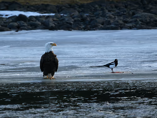
We used the following image to analyze the IG saliency map with the Swin Transformer model architecture. We did so because the image consists of two competing classes, Magpie and Eagle, both of which are learned by the STM. The STM model predicts the Eagle class for the image with a probability greater than 90% and the Magpie class with a probability less than 1%.
The explanation question to thus explore was: what regions of the image contribute to the model prediction for a given class? Furthermore, we wanted to test whether attributions, represented in the form of a normalized color map, for STM architecture with randomized parameters are any different from the saliency maps for the trained model.
The baseline tensor used for IG calculations was a gray image. IG computes the integral of the gradients of the model's output with respect to the input along a straight path from a baseline (gray image) to the input image.
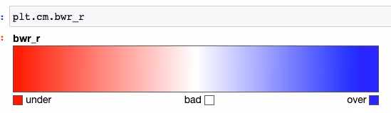
The following colormap was used where red represents negative and blue represents positive attributions. Thus, if a pixel is red it means that the pixel negatively influenced the model’s predictions. If it’s white it implies that the pixel did not influence predictions.
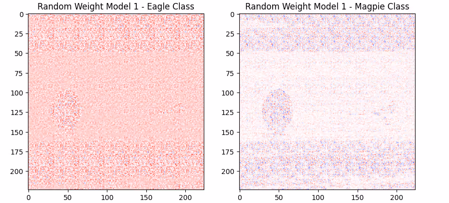
The following raw attributions for each pixel are plotted for the 224x224 image for a randomly initialized model with STM architecture.
If each image pixel is normalized by using the min attribution value and the max attribution value for the 224x224 image as a whole, we observe that the saliency maps generated for both images appear visually similar even though the raw attribution values plotted above have some color differences due to the actual attribution values being used.
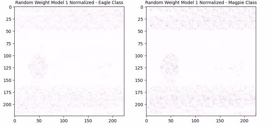
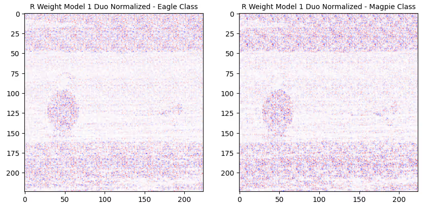
Further, if each image pixel is normalized by using the min of the two image mins and the max of the two image max, we observe that the saliency maps generated show subtle differences which were lost with individual normalizations. For example, for the randomized model 1, for the eagle class, you notice the eagle heads as an edge detected for the eagle class but not for the magpie class. Note: even though this model has randomized parameters and can be considered a “garbage” model, the focus of this exercise is more on the choices we make while illustrating image attributions and their deep impact on the way users of saliency tools may perceive/conclude the results of such an explainability tool. Similar observations have been made in the context of visualization of feature attributions for images13.
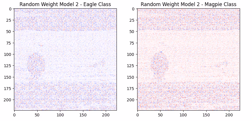
We repeat the above activity for a second randomly initialized model with STM architecture.
The following raw attributions for each pixel for model 2 are plotted for the 224x224 image
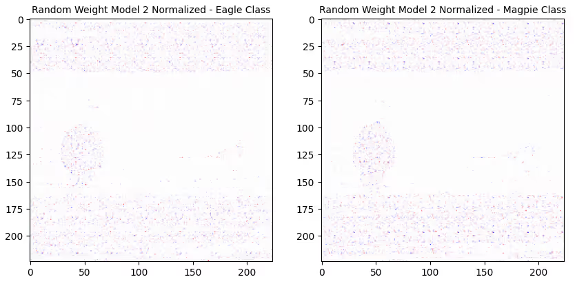
The individually normalized attribution values for the second randomly initialized model are illustrated below.
The normalized attribution values by considering both the images’ min max values for the second randomly initialized model are as follows.
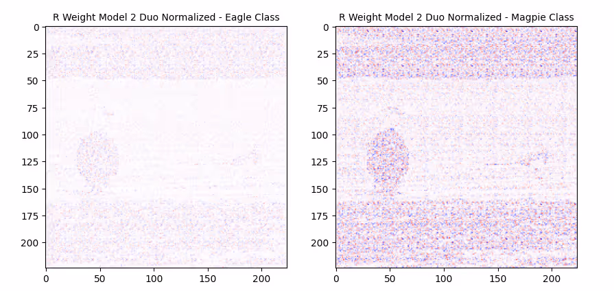
We note a similar trend with the attributions from the second randomized model where even though original raw attributions were different for each class, the individually normalized images appear the same. Further, when images are normalized by considering both of their attribution values, we notice the differences appear back again.
Now, we focus our attention on the actual STM with trained parameters. The following raw attributions for each pixel are plotted for the 224x224 image for the actual STM model with trained parameters.
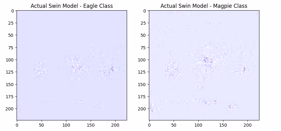
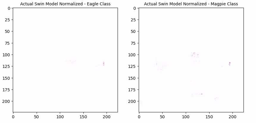
The individually normalized attribution values for the actual model are illustrated below.
The normalization by considering both the images’ min max values is illustrated below:
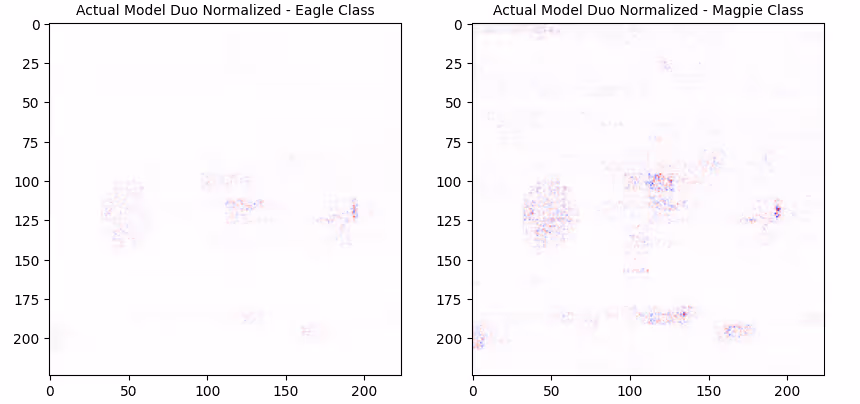
Note how the saliency maps of the actual model are very different from the randomly initialized model. We do not see the edges of various objects anymore. Further, there is a similarity in the trends of the explanatory power of the saliency maps dependent on the way the attribution normalization occurs. If images are normalized using their own min-max attribution values, the ability to gain an understanding of the regions the model is sensitive to decreases. However, when two images are normalized together, the ability to understand the saliency maps improves. Of course, the downside of this is that when class outputs are greater than two, we would need to consider pairwise k choose 2 visualizations.
In order to further elaborate on the differences between a randomly initialized model’s image attributions to that of the actual model’s attribution, we summed up the attribution values of the pixels within a manually drawn bounding box around the eagle [ x: [30,70], y: [100,150] ] and the magpie [ x: [160,200], y: [115, 130] ].
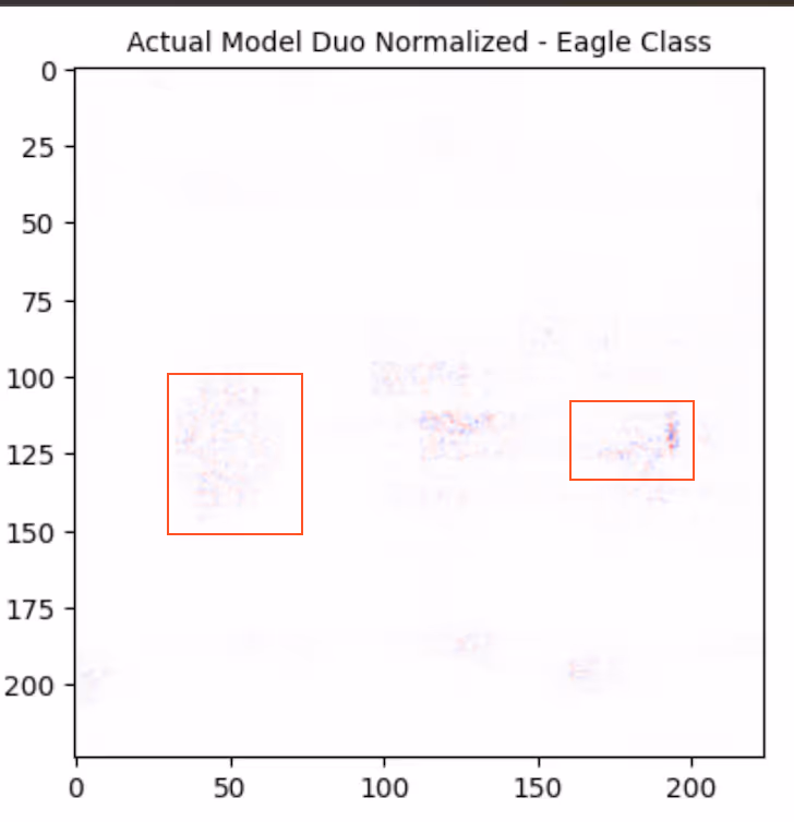
Here are the results:
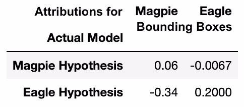
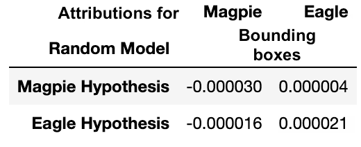
The summed-up attribution values represent how much the predictive probability deviates from the probability of a baseline gray image. A positive value of summed-up attributions for a particular bounding box implies that the region is enabling the model to become more positive for a particular hypothesis. Note that the summed-up attribution values for both the birds and both the class outputs are negligible for the randomly initialized model 1. Whereas, for the actual model, the values are comparatively significant. Furthermore, the summed attributions for the eagle/magpie negatively impact the prediction probability in the actual model for the magpie/eagle hypothesis. However, for the randomly initialized model that is not the case. These details are important while analyzing model explainability using attribution approaches and should be taken into consideration by the user. From a design standpoint, incorporating this information into the user interface (UI) is critical from a responsible AI perspective because such information in conjunction with the saliency maps reduces the chances for a misconception that might be developed if one were to only observe the saliency maps.
Similar results hold for other magpie images and eagle images. However, we chose the above specific image because of the presence of both competing classes of interest, that is, eagle and magpie.
Discussion
The results above highlight the need to train individuals to utilize saliency-based tools in a manner such that they are aware of the assumptions and potential pitfalls in interpreting explainability results solely on the basis of what they see. It is thus important for such tools to let the user know the design decisions made to illustrate the images/maps as well as let the user have the autonomy to manipulate the knobs of visualizations to be able to holistically understand the effect of image inputs on the model outputs.
Caveats to note while visualizing IG attributions as a heatmap:
- It is important to know if and how normalization was carried out to display the pixel attributions.
- It is important to know the min and max values of the attribution as well as the sum of the attributions of all the pixels.
- When comparing with another saliency map, it is important to account for max and minimum values across both images to get an idea of the relative differences.
Regarding randomization tests:
- We notice that two STM architectures with randomized parameters generate similar-looking saliency maps. However, the saliency maps from the trained model are quite different from models with randomized parameters. Thus, it might be unfair to make conclusions about saliency maps just based on the observed behavior on randomly initialized models.
- Explanations are faithful to a particular model in concern so it’s important to not conflate explanations from a particular model with another randomized model.
We note that saliency maps show us the important parts of an image that influenced the model's decisions. However, they don't tell us why the model chose those specific parts. On the other hand, attribution values indicate whether a certain region of the image positively or negatively contributed to the model's prediction, and they can be shown using different colors. But to avoid biasing humans, it might be better to look at the actual numbers instead of just relying on colors.
In conclusion, we have demonstrated that when using integrated gradients (IG) to generate saliency maps, two randomly initialized models appear to produce visually similar heatmaps. However, it is important to note that these findings do not necessarily apply to models loaded with trained parameters. While randomizing model parameters can be a useful approach to evaluate explanation methods like IG, we have emphasized that IG explanations remain faithful to the model. Dismissing the efficacy of IG based on the results of randomly initialized models may not be a fair assessment of the explanation technique. Additionally, we have discussed the significance of post-processing decisions, such as normalization, in generating accurate heatmaps and avoiding visual bias. Utilizing the pixel importance, specifically the min-max attribution values, across both compared images is crucial for a fair representation of the impact of each pixel. It is important to clarify the normalization effects to users to prevent human biases and misconceptions during the visual inspection of heatmaps and their attributions.
———
References
- David Gunning, Explainable Artificial Intelligence (XAI). Defense Advanced Research Projects Agency (DARPA), 2017.
- Wojciech Samek, Grégoire Montavon, Andrea Vedaldi, Lars Kai Hansen, Klaus-Robert Müller, Explainable AI: Interpreting, Explaining and Visualizing Deep Learning, Springer, 2019
- Christoph Molnar, Interpretable Machine Learning: A Guide for Making Black Box Models Explainable. https://christophm.github.io/interpretable-ml-book
- Riccardo Guidotti, Anna Monreale, Franco Turini, Dino Pedreschi, and Fosca Giannotti. A Survey Of Methods For Explaining Black Box Models, arxiv, 2018
- Kush R Varshney, Trustworthy Machine Learning, http://www.trustworthymachinelearning.com/, 2022
- Julius Adebayo, Justin Gilmer, Michael Muelly, Ian Goodfellow, Moritz Hardt, Been Kim, Sanity Checks for Saliency Maps, NeurIPS 2018
- Amirata Ghorbani, Abubakar Abid, James Zou. Interpretation of Neural Networks Is Fragile. AAAI 2019.
- Sara Hooker, Dumitru Erhan, Pieter-Jan Kindermans, Been Kim, A Benchmark for Interpretability Methods in Deep Neural Networks, NeurIPS 2019
- Himabindu Lakkaraju, Nino Arsov, Osbert Bastani, Robust and Stable Black Box Explanations, ICML 2020
- Muhammad Bilal Zafar, Michele Donini, Dylan Slack, Cédric Archambeau, Sanjiv Das, Krishnaram Kenthapadi, On the Lack of Robust Interpretability of Neural Text Classifiers, ACL Findings, 2021
- Mukund Sundararajan, Ankur Taly, Qiqi Yan, Axiomatic Attribution for Deep Networks, ICML 2017
- Liu, Ze, Yutong Lin, Yue Cao, Han Hu, Yixuan Wei, Zheng Zhang, Stephen Lin, and Baining Guo. "Swin transformer: Hierarchical vision transformer using shifted windows." In Proceedings of the IEEE/CVF international conference on computer vision, pp. 10012-10022. 2021.
- Krishna Gade, Sahin Cem Geyik, Krishnaram Kenthapadi, Varun Mithal, Ankur Taly, Tutorial: Explainable AI in Industry, KDD 2019